

The Bulk Update That Was Fast Until Nobody Ran ANALYZE
An application built on TypeGraph reported an import that was linear up to
5,000 rows and then fell off a cliff: 131 seconds at 10,000 rows and 482 at
20,000. One statement accounted for 107 of the 123 seconds of database time at
10,000. Running ANALYZE first brought the whole import back to 22 seconds.
That last detail is the interesting one. Nothing about the data or the query had changed. The only difference was what PostgreSQL believed about the table.
This post is about that statement, the three ways I failed to fix it, the one that worked, and the case the fix made slower. I am including the last part because a performance post that only shows the winning column is not much use to anyone deciding whether the trade is right for them.
Why the statistics were stale
Section titled “Why the statistics were stale”TypeGraph stores every node in one table, typegraph_nodes, keyed by graph,
kind and id. An application with many tenants ends up with a large shared
table and many small populations inside it.
PostgreSQL’s autovacuum re-analyzes a table once the rows changed since the last analyze exceed a threshold plus a fraction of the table: 50 rows plus 10% by default. On a table with a million rows, an import of 20,000 never gets there. So for the whole of that import, and for as long afterwards as the table goes without growing by a tenth, the planner’s picture of the new rows is whatever it can infer from statistics gathered before they existed. For a kind it has never seen in that graph, the inference is “about one row”.
The statement
Section titled “The statement”The import promoted the rows it had just inserted with one call:
await store.nodes.Version.updateWhere({ where: (version) => version.id.in(ids), patch: { active: true },});updateWhere() compiles the selection into a candidate query and wraps it in
one UPDATE. In the previous release it had this shape:
UPDATE typegraph_nodesSET props = ..., version = version + 1WHERE graph_id = $1 AND kind = $2 AND deleted_at IS NULL AND id IN (SELECT id FROM (/* candidate query */) AS candidates)The graph_id and kind conditions on the outer table are deliberate. They
are write fences: whatever the candidate query returns, the update can only
touch rows of this graph and this kind.
They are also what went wrong. With statistics saying the kind holds one row, the cheapest plan PostgreSQL can imagine is to walk that kind’s index range as the outer side of a nested loop and, for each row it finds, run the candidate subquery and check for the id. One outer row, one subquery execution: fine.
The kind actually held every row of the import. So the subquery ran once per
row, and each run produced the full candidate list. EXPLAIN (ANALYZE, BUFFERS) at 3,000 rows showed 3,000 loops of 1,500 rows, 4.5 million rows
discarded by the join filter and 12 million buffer hits, for a statement that
changes 3,000 rows.
It got worse before it got better
Section titled “It got worse before it got better”While that report was on its way, I had already made the statement slower on the development branch. It never shipped, but only because the report arrived first.
A fix there closed a real concurrency bug. Under READ COMMITTED, a row
that another transaction changed while the update waited for its lock was
re-checked against the outer conditions only, so a patch could land on a row
that no longer matched the caller’s predicate. The fix matched each candidate
with the version the statement’s snapshot had read:
AND (id, version) IN ( SELECT selected.id, selected.version FROM (/* candidate query */) AS candidates JOIN typegraph_nodes AS selected ON selected.graph_id = $1 AND selected.kind = $2 AND selected.id = candidates.id)That is correct, and it put a second copy of the same misestimated table inside the part of the plan that was being rescanned. Quadratic became cubic. With 50,000 analyzed rows of other graphs in the table, updating 1,000 fresh rows visited 167,668,500 rows and 4.1 million buffers. On the benchmark’s larger table the statement took 259 seconds for 1,000 rows, against a quarter of a second in the release before.
A correctness fix that is verified with fresh statistics tells you nothing about how it plans with stale ones. I now have a test for that, which I will come back to.
Three fixes that only moved the loop
Section titled “Three fixes that only moved the loop”Rewrite the join. A CTE, unnest over an array of ids, a LATERAL join:
each changes the syntax and leaves the planner with the same belief, that the
nodes table side is one row, and so the same decision to put it on the outside
of a nested loop.
Turn the candidates into an array. id = ANY(ARRAY(SELECT ...)) computes
the list once as an InitPlan, which sounds like exactly what is needed. But
with the constant graph_id and kind predicates still on the table, the
planner reads the kind’s range through that index and applies the array as a
filter on each row it fetches.
Split it in two. Read the candidate keys, then issue updates with the keys as bound parameters, so the planner knows exactly how many there are. This is the one I was most confident in, and an independent review took it apart:
- A row deleted and re-created under the same id between the two statements can carry the same version number, so the second statement patches a row the first never selected. One statement does not have this problem, because PostgreSQL’s re-check follows the row it locked, and a re-created row is a different row.
- On a connection in autocommit mode, a failure partway left the earlier chunks committed.
- It was still not linear. With the constant predicates in place, each chunk read the same index range and filtered it.
The common thread is that none of these changed what the planner was allowed to believe about the table. They rearranged the query around a wrong estimate.
What worked: take the constant away
Section titled “What worked: take the constant away”The fix keeps the update as one statement and moves the fences. The graph and kind stop being constant predicates on the nodes table and become columns of the key set the candidates are turned into:
WITH keys AS ( SELECT DISTINCT CAST($1 AS TEXT) AS graph_id, CAST($2 AS TEXT) AS kind, candidates.id FROM (/* candidate query */) AS candidates)UPDATE typegraph_nodesSET props = ..., version = version + 1WHERE deleted_at IS NULL AND (graph_id, kind, id, version) IN ( SELECT selected.graph_id, selected.kind, selected.id, selected.version FROM keys JOIN typegraph_nodes AS selected ON selected.graph_id = keys.graph_id AND selected.kind = keys.kind AND selected.id = keys.id )The fences are exactly as strong as before: a row can only be written if its
graph, kind and id all come from the key set, and the key set’s graph and kind
are the two parameters. What changed is that the nodes table now has no
constant range for a stale estimate to shrink to one row. It can only be
reached by joining on keys. DISTINCT matters here: PostgreSQL does not
flatten a DISTINCT subquery into its parent, so it cannot push the two
constants back down onto the table.
Any plan that avoids looking each key up has to scan the whole table, and a table scan is costed from the table’s real page count, not from column statistics. So the planner reads the candidates once and finds each target row by an index lookup on its id.
Measured by replaying the store’s own UPDATE under EXPLAIN (ANALYZE, BUFFERS), with stale statistics, identically on a PostgreSQL server and on
PGlite:
| Rows updated | Rows visited | Buffers | Buffers per row |
|---|---|---|---|
| 1,000 | 3,000 | 29,436 | 29.4 |
| 5,000 | 15,000 | 146,487 | 29.3 |
| 10,000 | 30,000 | 292,457 | 29.2 |
| 20,000 | 60,000 | 584,908 | 29.2 |
Three rows visited per row updated, at every size.
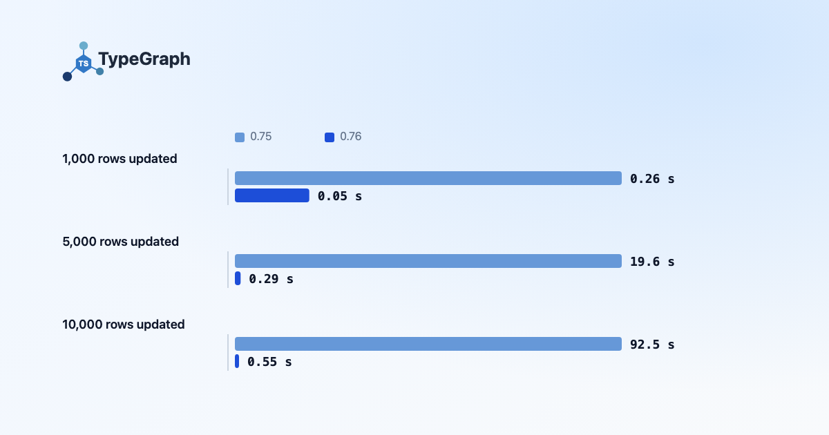
In seconds, for the UPDATE statement alone, on a table holding 300,000
analyzed rows of other graphs:
| Rows updated | 0.75 | 0.76 |
|---|---|---|
| 1,000 | 0.26 s | 0.05 s |
| 5,000 | 19.6 s | 0.29 s |
| 10,000 | 92.5 s | 0.55 s |
| 20,000 | — | 1.16 s |
A whole updateWhere() call, including the candidate read and everything the
store does around the statement, takes 0.35, 0.67, 1.37 and 2.80 seconds at
1,000, 5,000, 10,000 and 20,000 rows.
The case it made slower
Section titled “The case it made slower”Removing the constant predicates removed something useful too. With them, the planner could always fall back on the kind’s index range. Without them, when it believes there are many candidates, its alternative to keyed lookups is a hash join against a sequential scan of the entire table.
That happens in a second kind of staleness. Suppose the graph is already in the statistics, under other kinds, and the kind is in the statistics, in other graphs, but the two have never been analyzed together. PostgreSQL assumes the columns are independent and multiplies their frequencies. Against a table of 1,000,000 analyzed rows it estimated 62,479 candidates for a selection that actually had one. For 62,479 candidates a table scan is the right call. For one, it is 367 milliseconds where the old statement took 1.
For an updateWhere() over a whole kind in that state:
| Analyzed rows | Candidates | Before: rows visited | After: rows visited | Before | After |
|---|---|---|---|---|---|
| 50,000 | 1 | 3 | 50,003 | 0 ms | 12 ms |
| 50,000 | 4,000 | 12,000 | 62,101 | 288 ms | 208 ms |
| 1,000,000 | 1 | 3 | 1,000,003 | 1 ms | 367 ms |
| 1,000,000 | 4,000 | 12,000 | 1,012,101 | 269 ms | 546 ms |
| 1,000,000 | 20,000 | 60,000 | 1,064,101 | 1.27 s | 1.56 s |
The old statement was cheaper in every row of that table. Above a few thousand candidates the row writes dominate and the difference stops mattering. Below that, a call that updates a handful of rows pays one scan of the table, and a loop of such calls pays one scan each, until the table is analyzed.
I expected the scan to give way to lookups as the table grew. It does not, because the overestimate grows with the table.
Three things bound the damage:
- A selection that names ids is not affected. An id list is estimated from
the list, whatever the graph’s and the kind’s frequencies say. In the same
state, an update of 100 rows selected by
id.in(ids)and a property visited 300 rows of a 94,000-row table.compareAndSet()is keyed for the same reason. - The cost is one scan, never a rescan. The old failure grew with the square or cube of the rows updated. This one is linear in the table and does not grow with the update.
- Analyzing the table removes it. With fresh statistics the plan is keyed.
So the trade is a catastrophic case for a bounded one. I think that is right,
and it is a trade, not a free win. If you run many small predicate-only
updateWhere() calls against a large shared table straight after a bulk load,
this release is slower for you until the table is analyzed.
Two narrower limits are in the documentation with their measurements: ids that are reused under many kinds of one graph, which only happens with caller-supplied ids, and the candidate query of a single-row mutation, which can still scan a kind’s un-analyzed rows.
What I would do differently
Section titled “What I would do differently”Test plans with the statistics you will actually have. Every test of the correctness fix ran against a freshly created, freshly analyzed table. The plan tests added with this change build a table that has been analyzed, insert rows it has not seen, and then explain the store’s real statement against them. They run on a PostgreSQL server and on PGlite, and the numbers agree to within a handful of buffers.
Assert the property, not a proxy. My first plan test asserted that the plan contained no join. It passed while the statement still rescanned an index range once per chunk. The tests now assert what matters: an index lookup per key, every other read executed once, and ceilings on rows visited and buffers per row. One of them also had to be loosened, because it required the expensive plan it was meant to bound.
Ask what the planner is allowed to believe. Each failed rewrite kept the constant predicate and reorganized the query around it. The fix was to stop making a statement about the table that the planner could be wrong about. That is a narrower idea than “don’t trust the planner”. It is closer to: when a write names its rows, let the rows’ keys be the only way in.
If you load in bulk
Section titled “If you load in bulk”The fix makes one statement independent of statistics for the common case. It does not make statistics unimportant, and there are other writes that still plan badly on rows the table has not analyzed. Two things are worth doing on a large shared table regardless:
- Run
ANALYZEafter a bulk load when your database role allows it. On the benchmark’s table it took about 0.4 seconds for the nodes table at both 300,000 and 1,000,000 rows, since it samples. - Lower the analyze trigger for the TypeGraph tables so autovacuum reacts to an absolute number of changed rows, not a fraction of a table that keeps growing:
ALTER TABLE typegraph_nodes SET (autovacuum_analyze_scale_factor = 0, autovacuum_analyze_threshold = 10000);ALTER TABLE typegraph_edges SET (autovacuum_analyze_scale_factor = 0, autovacuum_analyze_threshold = 10000);That shortens the window to one autovacuum pass after ten thousand changes, whatever the table’s size.
Further reading
Section titled “Further reading”- Stale statistics on a large shared table: both states, every measurement, and what is and is not affected
- Refreshing planner statistics after bulk loads
- The change itself, with the full measurement tables and the benchmark that produced them
- GitHub
Stay in the loop
Occasional updates on new features, guides, and releases. No spam.